Evaluating a classification model is generally straightforward: compare predicted outputs with the ground truth labels and derive a metric, such as an F-score. Got probabilistic outputs? No problem, just pick the most likely label (i.e. argmax it). Got a multi-label problem on your hands? Well, now you have to pick a threshold above which to consider each class label a positive. Still… not a big deal. The best threshold can be derived by, for example, calcluating a ROC curve, and finding an inflection point.
But here there be dragons. That ROC curve implies, again, the ability to compare the predicted labels against ground truth. The problem is…

If you’re lucky, your “ground truth” labels are already binarized 0/1 values. But real-world data comes with error. Maybe 3 different crowdsourced workers labeled each example, and maybe they didn’t agree. Maybe they had differing confidence levels. Maybe the class was ambiguous to begin with. So what do we do about thresholding the “ground truth”?
Ok, enough blah blah blah. Let’s code.
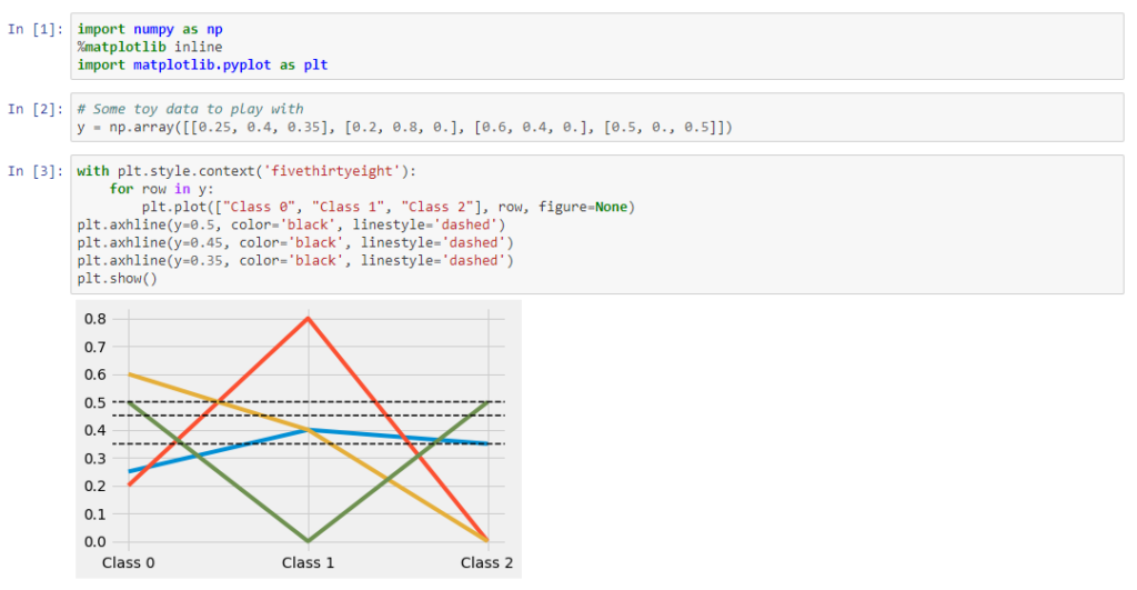
In the chart above, there are three example thresholds. All have different implications in terms of class membership, even in this small dataset, and all hover around 0.5 (a common and intuitive default). No strawmanning extreme values here (though we will evaluate them later, just to say we did). Which one of these is best?
We need a means to estimate ground truth with respect to our selection threshold. Statistical estimators that can take into account the different threshold possibilities applied to the provided probabilistic labels can be brought to bear. One such approach is outlined in a paper by Bart Lamiroy and Tao Sun, “Computing precision and recall with missing or uncertain ground truth.” Lamiroy and Sun present a system that applies a set of partitioning functions, S, to a set of documents, Delta. They derive a formula for precision and recall, which we will use here. Check out the paper for full derivation and experimental results!
In order to solve the problem of threshold optimization, we will take S(i) to be the result of applying candidate threshold, i, in [0..1] and Delta to be the binarized, flatted* output of applying that threshold to each implied prediction.
*Since we’re dealing with multilabel classification, we flatten out the above predictions to simply be a 1 or 0 indicating whether a specific combination of S, y (a given “soft” label, of which we have 4 above) and class (we have 3). In tensor terms, we move from a shape of (len(S), len(y), num_classes) to (len(S), len(y)*num_classes).
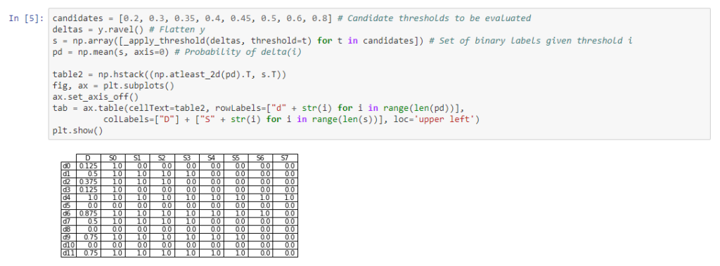
With these dimensions in hand, we have above a faithful replication of Table 2 from Lamiroy and Sun. Again, S(i) represents a choice of threshold (ranging from 0.2 to 0.8) and d(i) represents the class membership prediction for (flattened) document/class pair i.
Below, we use the precision and recall formulas from Lamiroy and Sun and derive the F1 as a combined metric. From here, finding the best F1 leads us to the optimal threshold (from among the candidate choices).
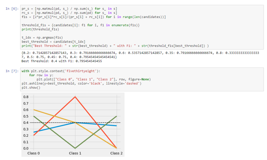
And with that, we have an optimal threshold with which we can binarize that data. There may be no such thing as ground truth, but now we have “ground truth”.
– Greg Harman, CTO