


So you’ve trained yourself a machine learning classifier. You want to tweet it (or whatever the kids do these days) to the world! Print out a copy of the weight matrix for Mom to hang on the fridge. But then self-doubt sets in. Is this classifier good? Could it be better?
How do we evaluate classifiers anyway? Some quick Googling will fill your browser tabs with introductory articles on F-scores, precision, recall, Type I/II errors, and so forth. While it’s tempting to pad this post (and add some pretty equation graphics to boot), I’ll refrain. Go ahead and check that stuff out. I’ll wait.
Back yet? You probably ran across confusion matrices; 2×2 matrices are the tried-and-true way to illustrate those metrics. We’re going to use this as a jumping-off point. Just for fun, we’ll use 3 classes, because binary classifiers are just so… yawn. Here’s a confusion matrix for an ideal version of our classifier.
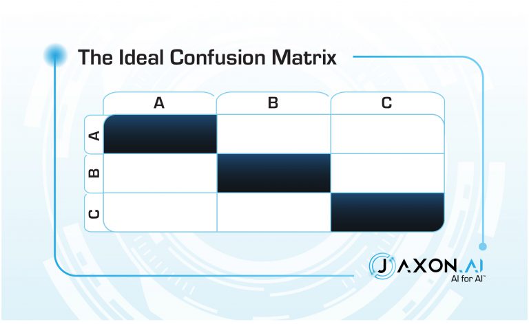
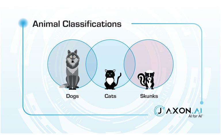
Too bad yours doesn’t look like this1. Confusion matrices are a great means of getting a quick visual of the quality of a classifier, and they can also be used as a guide for how to improve that classifier. Example, you say? Thought you’d never ask. Cute animals are always a crowd-pleaser, so let’s classify them.
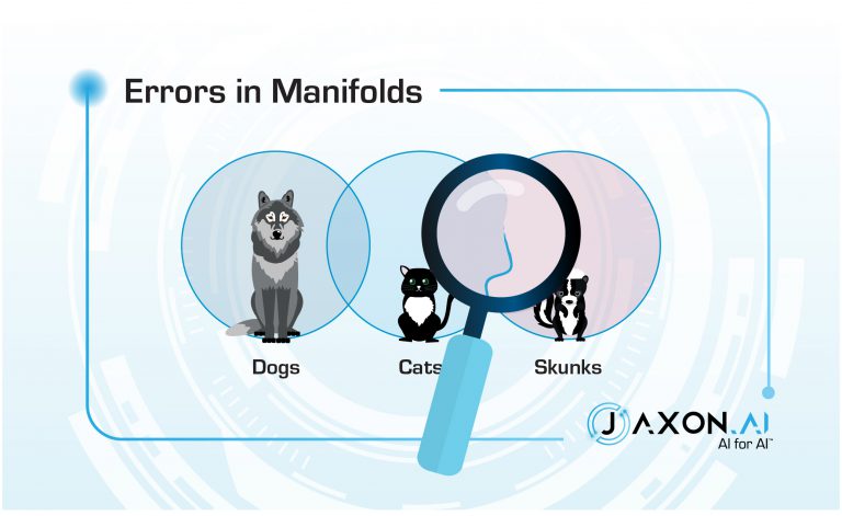
If you squint at them in just the right way, you can pretend that they are straight lines – these are called manifolds. Machine learning techniques commonly use manifold approximations to sort out the boundaries. Errors – that is, confusion – tend to be in places where the assumed manifold didn’t quite jive with reality. Data points near one of these manifolds are easily mis-classified.

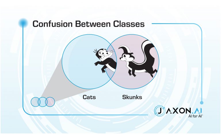
Example: Pepé Le Pew is convinced that Penelope Pussycat is a skunk. Penelope has no confusion as to Pepé’s class membership.
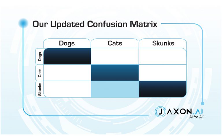
So each square in the confusion matrix is representing how much error exists across a specific manifold between two classes. We can use this intuition to improve our classifier.
How do I do this, you ask. Good question – you’ve probably already used all the (labeled) data you have, and tried out a few different algorithms, architectures, and parameterizations, and you’ve kept the best of the bunch.
One approach is to address the data. Yes, I know you used what you had, but did you try:
-
- Over-sampling examples around the confusing boundary?
- Going and finding new data focused on just that boundary?
- Generating synthetic data based on the two confusing classes?
These can be repeated strategically to help “zoom in” on problematic boundaries. If you’ve got a specific budget with respect to labeling examples, you might consider not spending it all initially. Hold some back to invest into more labeling just around the trouble spots. How can I find just those since my data spans all classes? Well you’ve got a classifier already! Grab (previously unlabeled) examples that are labeled with either class in question and relabel those.
All right, I get it. Maybe you just don’t have any more data available. And besides, labeling data is boring and takes a long time, and life is just too short. I agree. It’s time for those lazy machines to earn their keep.
The original model you’ve trained has already learned what it can learn from the data that we have available. But it has a disadvantage: it has to generalize across all classes. Jack of all trades, and master of none. What we need to do is give Jack a team to help him out.
Consider training specialist models—binary classifiers, perhaps—to address just the most problematic boundaries. These might take the form of anything from advanced deep-learning models to simple human-coded heuristics; anything that can help discern that specific boundary.
These can then be used to augment the original “main” model. This might take the form of a flat aggregation scheme like Snorkel or majority votes, or maybe be a confidence- and class-triggered branch: if the main classifier predicts skunk and confidence is below 80%, then use the specialist cat-vs-skunk classifier, else keep the original prediction.
Or, you might use this specialist classifier indirectly, combining it with data augmentation. Use it to label some new (previously unlabeled) training data, and then combine that with the original training data to re-train the primary classifier.
The devil is in the details, of course, and noisy labels carry additional challenges, but that rabbit hole goes deep and I’ve met my word count quota. I hope that this post has inspired you to view confusion matrices not as passive after-action measurements, but as a tool that can help you actively improve your models.
– Greg Harman, CTO
1 Unless you cheated and let your validation data leak into your training set.