


Splitting Datasets
As we train machine learning models and prepare our training data, one of the first questions that comes to mind is “How am I going to split off a test set so that I can measure the models that I produce?” There’s a rule of thumb that most of us use, which is to take our data and randomly split off 20%.
But is a rule of thumb like that always the right answer? “Always” should set off alarms because there’s just about nothing that always works. On one hand, if you make your test set too big, you’ve wasted examples that could have made the model perform just a little bit better. Conversely, if it’s too small, it will be a poor measurement of your model’s performance once it rolls out into the field. You simply haven’t covered all the potential cases—they’re single measurements out of a distribution you can’t see. Are you getting the distribution towards the middle of that mean (and how big is that distribution), or are you taking something that’s less representative?
Over- and Under-Splitting
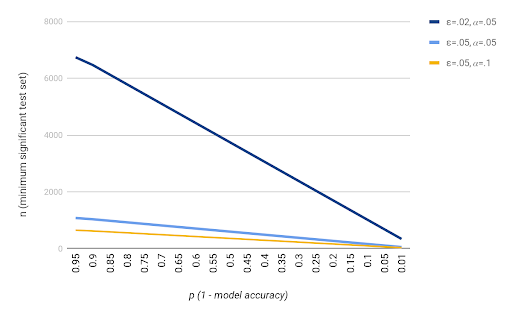
Before we even talk about how to split it—if we still assume a random sampling—how much should we split off? First, you have to establish a confidence bound. You can’t have a magic number that’s always right, but you can say that, within a certain degree of error, you’re willing to tolerate a given measurement in a particular confidence bound. A typical choice is a 5% error within a confidence of 95%.
When you start to assemble for a given dataset and model, you first ask, “How many examples do I need in my test set to be sure I meet those conditioned bounds?” While you won’t know that until after you’ve trained it, you’ll at least have some idea of its general accuracy. The more accurate your model is, the fewer examples you’ll need to verify. If you have a model that’s supposed to be 99.999% accurate, one wrong answer and you’ve pretty much thrown that out the window, whereas if your model is 50% accurate, you’re going to have to measure an awful lot before you’re sure.
Types of Drift
We’ve talked about how to split off your data and how big your test set needs to be, but that sort of under/over splitting is not the only thing that can go wrong when it comes to splitting off your data and making sure that your model evaluations are accurate. Other things happen—data changes. There’s all sorts of drift.
The notion of the environments of your data—which is a subtle way to describe the nature of your data (e.g. what are the examples like, are they changing over time, are they changing with context as you measure it in different systems, are the predicted values changing?).
Sometimes it might be the master set, the range of values or, the distribution. Maybe you’re just naturally starting to see a few more dogs than cats, or there are more dogs than cats in your dataset. Or maybe dogs are outperforming cats in the world because, as we all know, dogs are better. And conversely, if you have a very small sample, you can get bias—particularly for test sets, but that’s also true for training sets and other sample tests.
Concept Drift
One of the ways that data may change over time is concept drift. This story was originally told by Google in a paper called “Invariant Risk Minimization”. Some researchers want to create an image classifier that separates cows from camels. They bring up a great classifier and roll it out to the field, and it starts misclassifying when they start taking live pictures. Why?
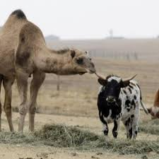
Well, in this case, the training data contained a bias that nobody had considered—all the pictures of camels were taken in a desert with a brown background, and all the pictures of cows were in pastures with a green background.
As soon as the classifier ran across a picture of a cow standing on dirt or a camel standing on grass, it would misclassify. They’d accidentally trained a background classifier.
Invariant risk minimization is one of the primary ways to deal with this drift. The idea is to introduce an intermediate stage into your data—instead of predicting your outputs (cow vs camel), you find an invariant representation. You’re searching for a function such that, when we transform a variable, it will still make the predictions you want even as conditions change.
Probability Drift
We also have to consider probability drift, where we have the same variables with changing distributions. Maybe people are selling all their cows to buy camels. Or maybe you’re modeling a town’s housing prices over time. You can build a very accurate and effective model for housing prices in 1950.
Fast forward it to today, 70 years later, and that model won’t help you at all. The prices have changed according to inflation, land, proximity to locations like airports, and etc—and they haven’t necessarily gone up proportionately.
Time is the primary dimension where drift occurs. The best way to deal with this is to simply monitor and adjust. No model stays as accurate as it was in the beginning of its lifespan. These are living things, so to speak, and they need to be continually monitored and fed with new, updated examples and adjusted as biases start changing. Eventually, the models need to be updated or replaced with newer models trained on newer data.
Covariate Drift
Now we get into the part of the world that Jaxon’s SmartSplit technology is really designed to address. In the case of covariate drift, the probability of a variable—the distribution of cows and camels, or median house prices—isn’t going to change, but the probability of what we’re going to see in the actual data does.
Think about language: we haven’t used ‘thou’ since about the 17th century. Let’s say you want to figure out if Shakespeare could have written a certain passage. Does it have the word ‘thou’ in it? Then maybe. Does it not have ‘thou’ in it? Well, he probably used that, given he was writing before the 17th century. SmartSplit is designed to help with this sort of covariate drift, where the distribution of a variable’s latent features changes over time, but the distribution of our output does not.
Covariate Drift and SmartSplit
For example, our slated task here is a dataset that we want to divide up by some proportion. We want to figure out which specific examples from the dataset should go into the training and test set, and if we can do better than random sampling.
Random sampling fails because all the examples are not created equal. Some of them will be duplicates. Some of them will expose more than one latent feature that the system might be able to find signal in. And some of them aren’t that useful at all. We want to make sure that we are very choosy about exactly which representations go into which bucket, even in the dimensions that we haven’t been able to see.
The three high-level steps of SmartSplit are:
- First, create a representation. This could be something inspired by the invariant risk minimization that we talked about, but it doesn’t have to be
- Once we have projected our dataset into this representation space, we’ll create a strategic clustering chain over that. We’re going to further subdivide those examples into clusters, each of which focuses on a particular topical area or latent feature subarea.
- Finally, when we do our split, we’re going to sample those clusters, ensuring that everything comes back out with the expected distribution. So if we want an 80/20 split, for each cluster, we’ll take 5 examples and put 4 into the train set, 1 into the test set.
The Payoff from SmartSplit
Let’s dig in a little deeper and see the results. There are two primary benefits of using SmartSplit:
The first one, and the reason we started looking into this, is the notion of test variants. When you take one test set to evaluate a model, you’re getting a single measurement of that model’s theoretical distribution over all the documents that it see in production. Your model’s accuracy is actually more like a distribution, and you’re taking one measurement of its performance against its performance distribution with the test set. If we can reduce the variance of that curve, then we can ensure that we’re more accurately measuring that model’s true performance output.
The additional piece here is that… How can we split the data such that the measurement we make on a model is more likely to reflect its performance in production, and thus avoid the traditional disappointment of watching a model that performs great in the lab fall flat the moment it hits production?
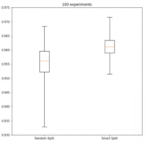
We’ve had some very encouraging success. Below, there are two graphs of different benchmarks we ran, each of which represents a different dataset and modeling problem. We ran the same problem, including random splits, on the left side and SmartSplits on the right side. In both cases, the SmartSplit distribution on the right side is narrower than the random split on the left. When we add up the numbers, we’re getting about a 3X reduction in variance with SmartSplit. That seems to hold up fairly well across datasets. We consider that a win!
Even More Payoff
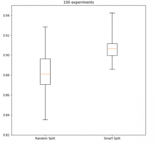
It turns out that not only is the variance better, so are the models. If you look at the image below, not only is the distribution band much smaller for the split compared to the right, but the mean/median/average output of the model (represented by the red lines) are also higher. We’re getting an average of 15% reduction in model error, which we hypothesize has to do with the fact that the model is seeing accurate proportions of the different types of latent feature spaces available in the training data. And if that wasn’t enough, our models are achieving convergence faster too.
– Greg Harman, CTO (Adapted from Jaxon’s SmartSplit Webinar)